

A Deep Dive into NVIDIA Rubin CPX: History, Architecture, Splitwise/DistServe, Inference Economics, and Limitations
A first principles analysis of why NVIDIA decided to make this new class of accelerator

Introduction
The Grace-Blackwell CPU + GPU couplet will be succeeded by the new Vera-Rubin platform. In addition to the LPDDR-based Vera CPU and the HBM4-based Rubin GPU, there’s now a third processor in the mix: the GDDR7-based Rubin CPX.
The idea behind this new processor is straightforward — make inference cheaper for providers while improving performance for users. This is done by separating the two stages of LLM inference, prefill and decode, and have the CPX run the prefill step and let the Rubin GPU run the decode step.
At GTC in March 2025 NVIDIA released Dynamo, their new inference framework, which makes disaggregate inference a first-class citizen and at the AI Summit in September 2025 they announced Rubin CPX. This marks NVIDIA’s firm commitment towards this disaggregated model of inference.
In this article, we’ll take a step back and analyze from first principles:
The core issues with LLM inference and what are prefill and decode.
Why separating prefill and decode helps, and the research that uncovered these optimizations.
Then we’ll walk through the Rubin CPX architecture, examine its capabilities, limitations, and compare it with Blackwell and Rubin GPUs.
What makes LLM inference difficult
Quality of Service
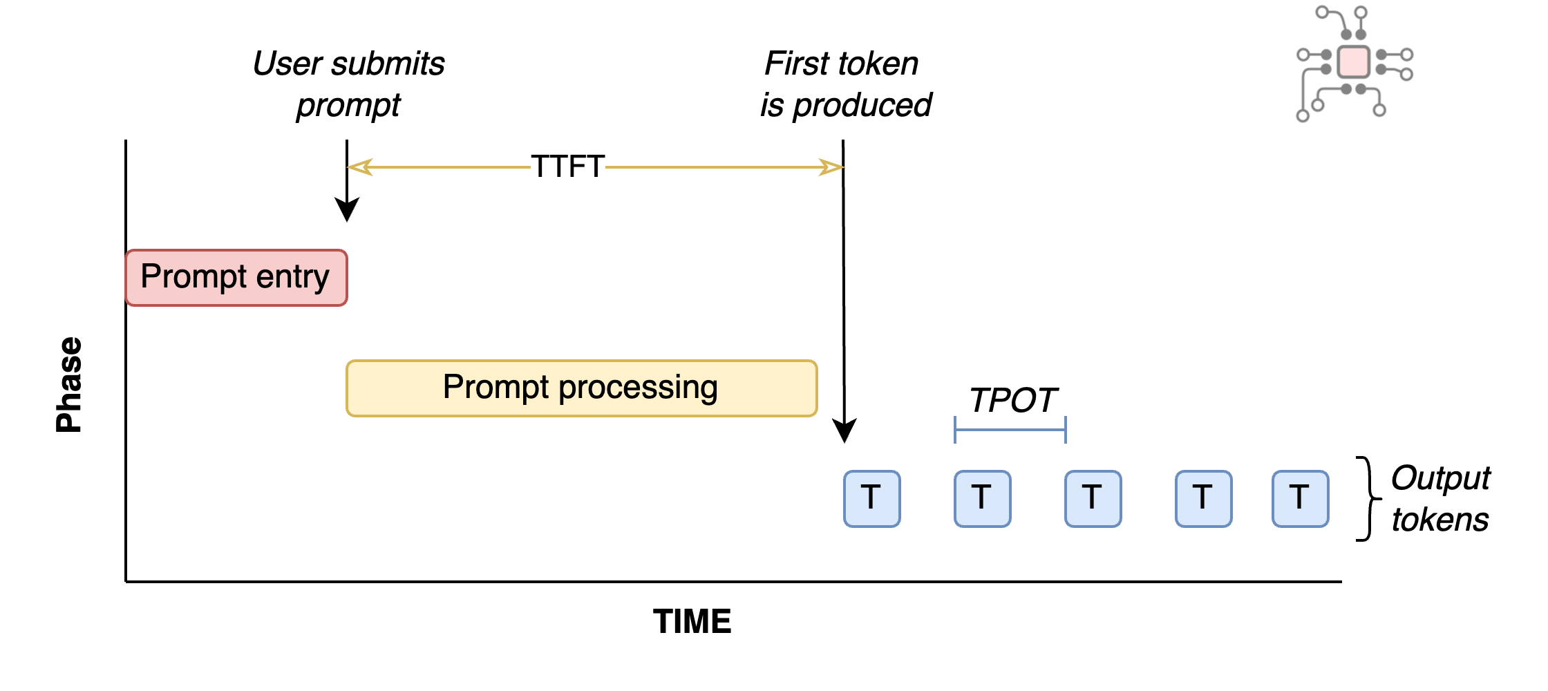
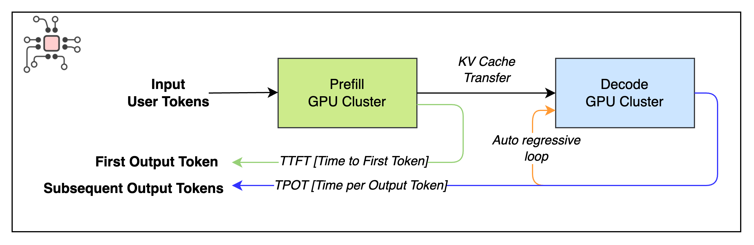
If you’re a paying user of ChatGPT, Gemini, or Claude Code, you have certain expectations about how responsive the service should be. The industry term for these expectations is called Service Level Agreement (SLA). For LLMs, two metrics determine whether that SLA is being met: Time to First Token (TTFT) and Time Per Output Token (TPOT).
These metrics are fairly intuitive. In a chatbot, TTFT is the time between submitting a prompt and seeing the first token appear. This phase of of processing is called Prefill. While TPOT is the speed at which each subsequent token is generated. This is the Decode phase.
Different applications have different requirements. A chatbot like ChatGPT needs a fast TTFT so the response feels immediate, but TPOT only needs to keep up with normal reading speed. In summarization, users tolerate a slower TTFT, but once the summary starts, they expect the rest of the output to appear quickly, so TPOT matters more. With tools like Claude Code, both TTFT and TPOT need to be fast.
What complicates things further for inference providers is that memory and compute demands vary dramatically across applications. The size of the input, (prefill phase) and the amount of output (decode phase) can differ by orders of magnitude. Text-to-image prompts are short but produce large outputs. Summarization and code generation often have long inputs but shorter outputs, and chat sits somewhere in between.
Economics
Managing the economics of LLM serving while meeting SLA is tricky. Different workload shapes from different customers make it hard to use the same hardware efficiently without breaking someone’s SLA.
For simplicity, imagine OpenAI is running ChatGPT on a single NVIDIA H100. To maximize profit, they want to serve as many user requests as possible on that one GPU while still meeting TTFT and TPOT targets. That effective “packing” of users per GPU is the batch size. If they try to fit too many users, latency spikes and people get frustrated. If they’re too conservative, they end up needing a prohibitively large GPU cluster to serve their millions of users.
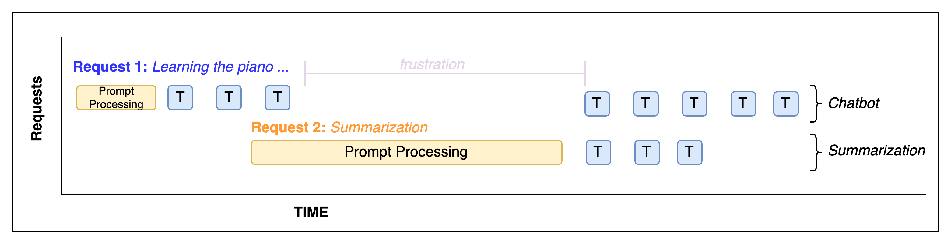
To make things worse, you don’t always need many users to overload a system, you just need the wrong mix. Even with just two users, one user might ask, “I want to learn the piano. Give me step-by-step instructions and resources.” At the same time, another user uploads a 50,000-word document and asks for a summary. On a shared GPU, your TTFT might look fine, but once the long summarization request arrives, your TPOT can get hammered, and you’ll see a noticeable pause in the middle of your chat.
So in order to maximize revenue while meeting SLAs and keeping users happy, we need to do two things:
Understand how different applications stress the GPU, i.e., what their workloads actually look like in terms of compute and memory
Find an efficient way to batch and schedule these requests so we can get the most throughput out of the hardware while still hitting TTFT and TPOT targets.
How we got to today’s LLM inference
Next, we’ll look at how LLM inference has evolved over the years through the lens of four seminal papers. These papers offer valuable insights, and understanding what they uncovered is key to seeing the path that led to Rubin CPX.

ORCA: 2022
Paper: ORCA: A Distributed Serving System for Transformer-Based Generative Models

Key innovations:
  - Iteration-level scheduling
  - Selective and continuous batching
Inference serving systems usually have two parts: an inference server or scheduler, which receives and batches user requests, and an execution engine, which issues kernels to the GPU.

For models like ResNet, used in image recognition, this setup is simple. Every request is a single forward pass through the network, all inputs have the same shape, batching is trivial, and the end-to-end latency is predictable. When the batch is done processing, the users get their responses. This is called request-level scheduling.
The authors of this paper showed that when you apply this kind of request-level serving system to LLMs, where each request varies widely in length and compute time, you run into two major problems.
For instance, in a setup with NVIDIA Triton (as the server) + FasterTransformer (as the execution engine), if three user requests were batched together, even if one finished early, that user wouldn’t get a response until all jobs in the batch were done.
If new requests arrived while a batch was running, they had to wait for the entire batch to finish before being scheduled, even if there were empty slots available.
The diagram below shows how these issues lead to high latency and poor GPU utilization, but the bigger consequence is its implication on cost of inference.
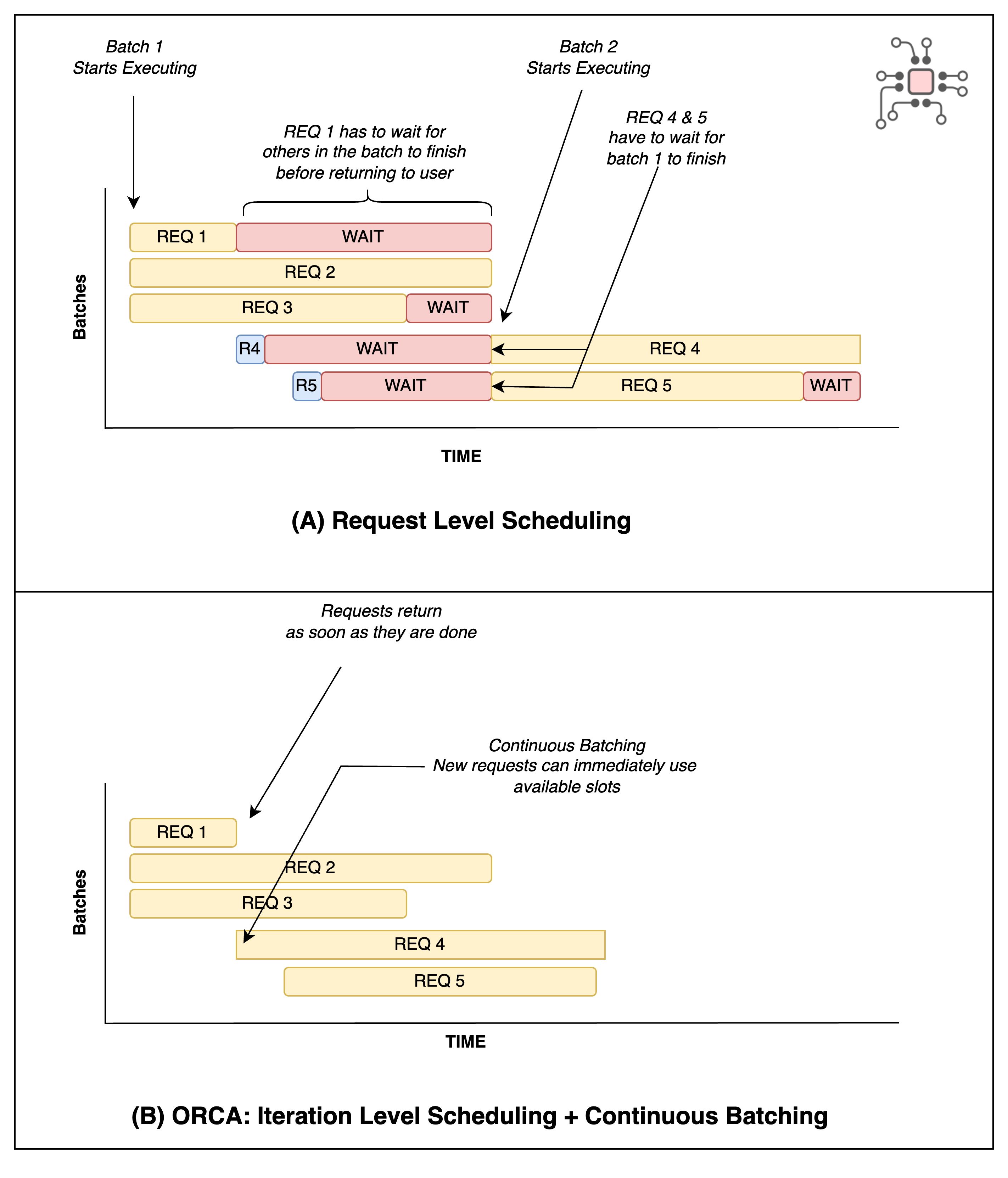
ORCA replaced request level scheduling with iteration level scheduling, so batching happens on a per-token basis instead of per-request. So when a user’s job is done, it returns immediately. This also allowed new requests to be batched in continuously as older ones relinquished their slot.
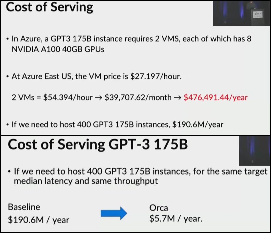
Fixing these issues increased throughput. With ORCA, the cost to run a GPT3-175B model, running on 2 nodes each with 8 x A100 GPUs, went down from $476,000/month to $14,000/month.
SARATHI: 2023
Paper: SARATHI: Efficient LLM Inference by Piggybacking Decodes with Chunked Prefills

Key innovation: Chunked prefill
This paper built on ORCA and reduced inference costs by another 25%. The key insight was that the prefill and decode stages have very different compute utilization patterns. Prefill can saturate a GPU even with a single request, while decode only becomes compute-efficient at large batch sizes. In other words, prefills were efficient, but decode suffered from poor GPU utilization.
Another issue in ORCA was, even within an active batch, there was some serialization happening, the requests were not parallelized efficiently. This caused “bubbles”, especially when a large model was split across GPUs. ORCA itself acknowledges this limitation, and this paper focused on addressing it.
SARATHI split each prefill into equal-sized chunks and built batches containing one prefill chunk and multiple decode requests. With this setup, during inference, the prefill chunk fully saturated the GPU, allowing the decode requests to “piggyback” at a much lower cost, up to an order of magnitude cheaper than running a decode-only batch.
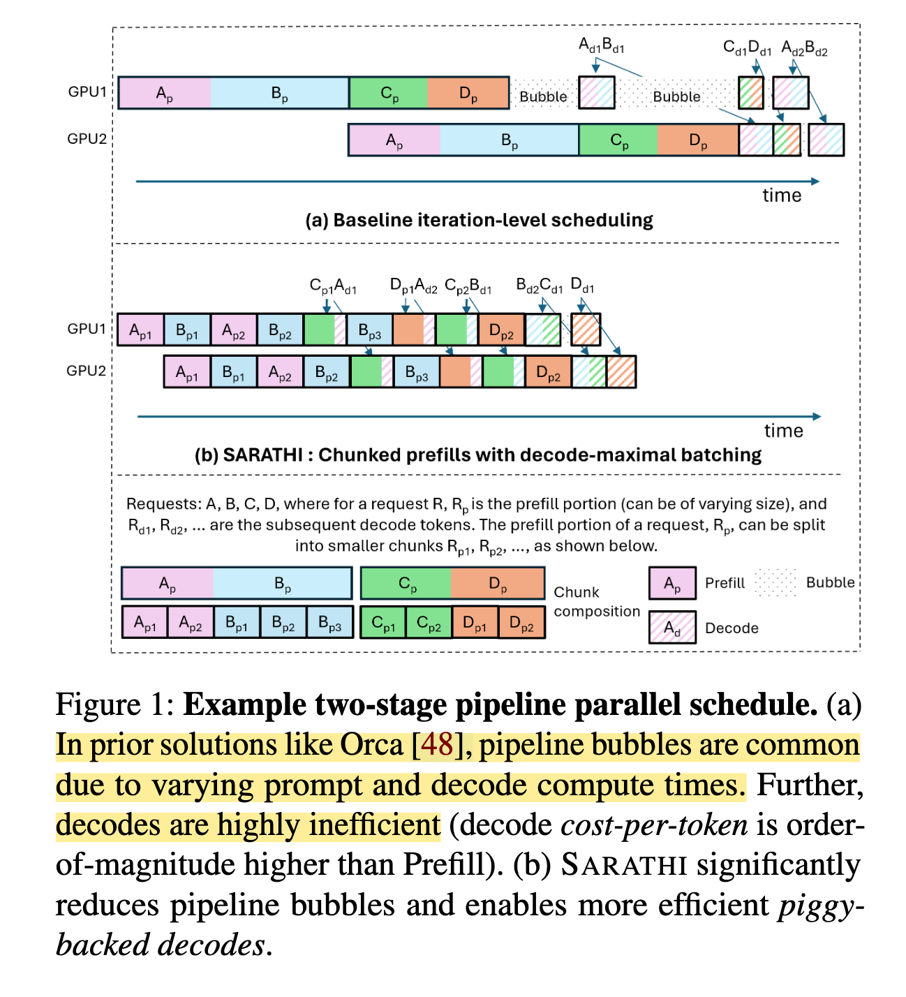
Although SARATHI improved decode throughput by up to 10×, it introduced one drawback. Chunking made prefills slower. As a result, the overall speedup over ORCA was only about 1.25×. Here’s how the paper describes it:
We note that although we improve decode efficiency by up to an order of magnitude, the end-to-end speedups and in turn monetary savings in inference cost are in the order of [only] 25%. This is because our technique only improves decodes and not prefills.
Splitwise & DistServe: 2024
Papers: Splitwise & DistServe

Key innovation: Disaggregated prefill and decode
This brings us to the two papers most relevant to Rubin CPX: Splitwise and DistServe. These parallel efforts showed the benefits of fully disaggregating prefill and decode and running them on separate GPU clusters. Splitwise demonstrated that disaggregation can deliver up to 1.4× higher throughput at 20% lower cost compared to SARATHI, or 2.35× more throughput under the same power and cost budget. They also showed that the decode phase can run on less compute-capable hardware with better perf/W and perf/$.
The authors of Splitwise clearly captured the impact of disaggregation. Their baseline was the standard setup where prefill and decode run together on A100 or H100 GPUs. They then compared this against configurations where prefill and decode were split across different machine types. The two charts below show throughput under iso-power (same power budget) and iso-cost (same server and operating cost). My annotations explain how to read them.
Machine combinations simulated:

+ A100.Prefill + A100.Decode
+ H100.Prefill + H100.Decode
+ H100.Prefill + A100.Decode
+ H100.Prefill + H100Cap.Decode (H100 cluster for decode were power capped).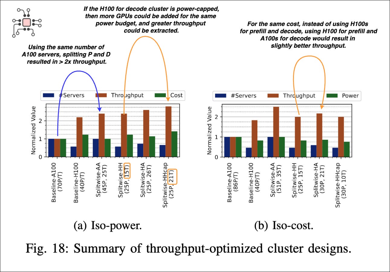
DistServe contributed additional ideas. Given a model, workload, latency target, and machine types, their algorithm determines how many machines to allocate for prefill and decode and what parallelism strategies to use for each of them.
KV-Cache transfer
One inherent overhead in disaggregation is KV-cache transfer. After the prefill cluster processes the prompt, the KV-cache must be moved into the decode cluster’s memory. Both papers analyzed this cost and proposed strategies to reduce its impact.
NVIDIA Dynamo: GTC 2025
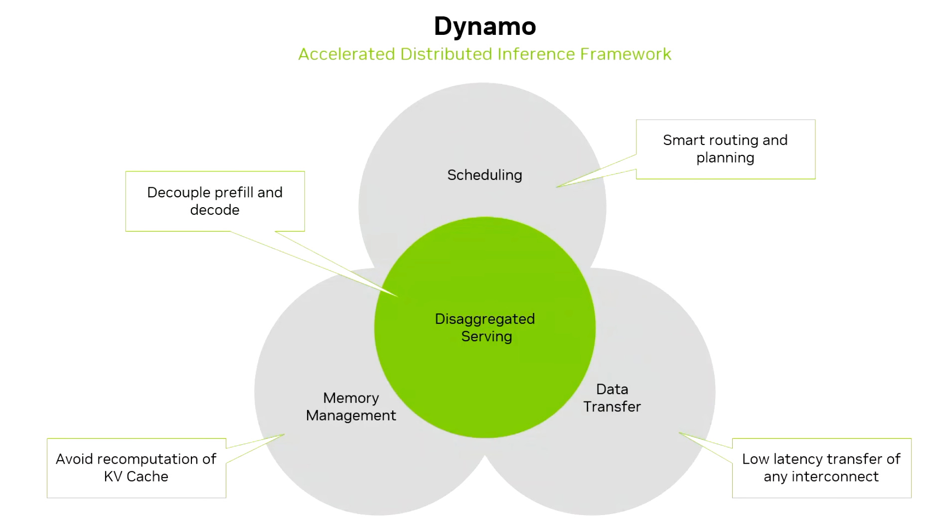
Finally, in March 2025 at GTC, NVIDIA announced Dynamo, their new inference framework. Like ORCA, Splitwise, and DistServe, it acts as the orchestrator, bringing together many of the ideas from these papers and adding several new capabilities of its own.
Notable:
In the GTC session, NVIDIA mentioned that, in 2024 and 2025 they met some Chinese customers who were pairing H800 GPUs for prefill and H20 GPUs for decode and that brought a lot of cost savings.
Some of Dynamo’s key features include:
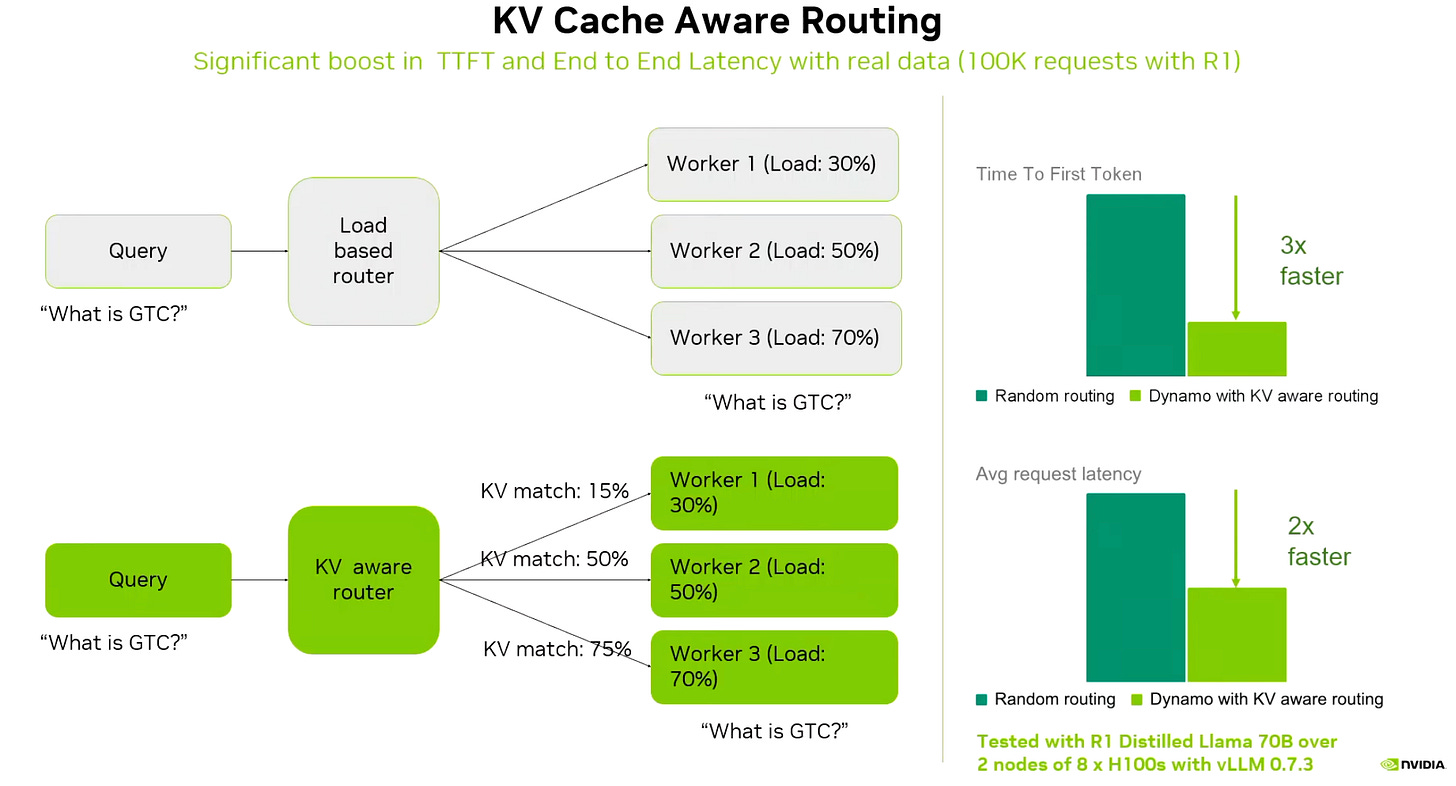
KV-cache aware request routing, which sends user requests to the right deployment cluster based on cache locality.
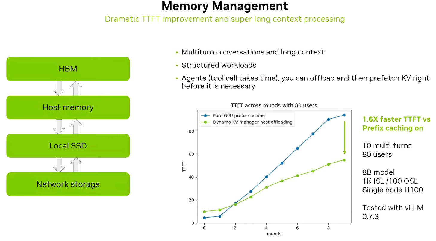
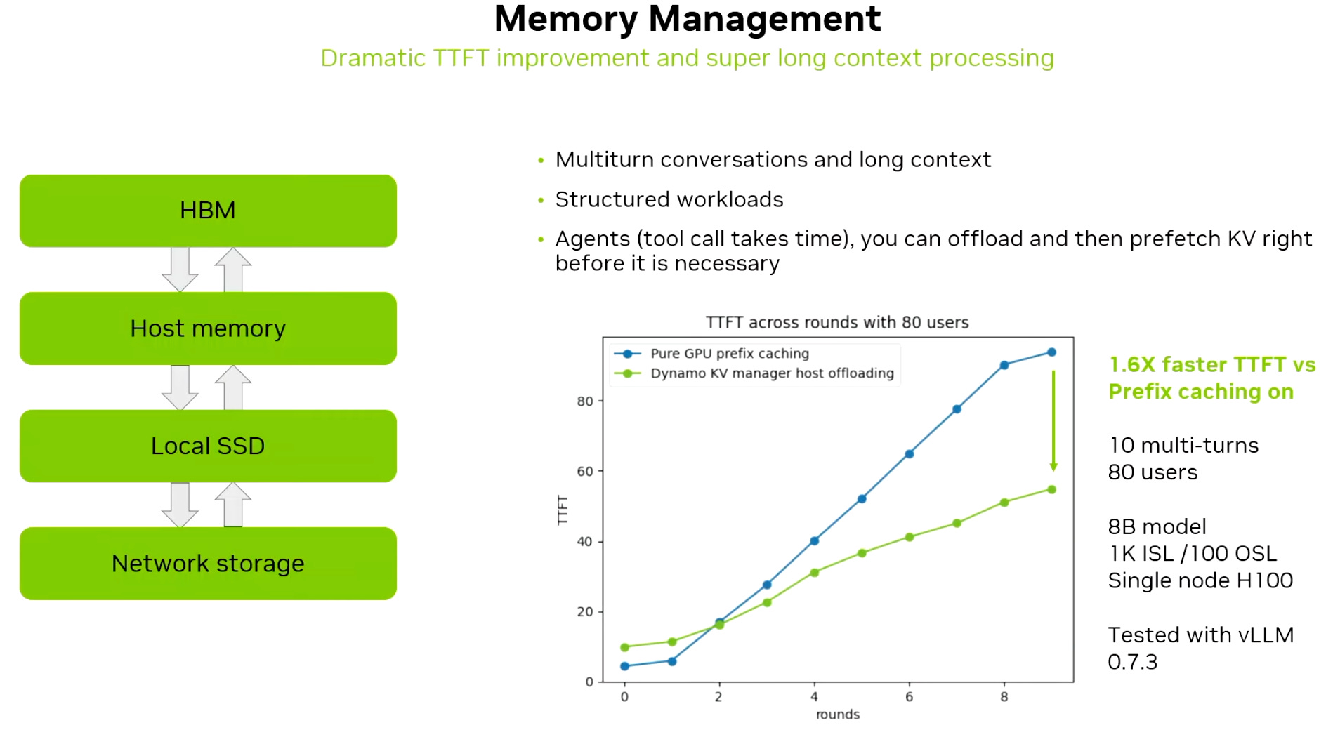
Source: NVIDIA (GTC 2025) A KV-Block Manager that can offload and retrieve KV-cache, significantly improving performance for workloads like code generation and multi-turn conversations.
Source: NVIDIA (GTC 2025) Production-grade serving tools, including fault tolerance and auto-scaling for separate prefill and decode clusters.
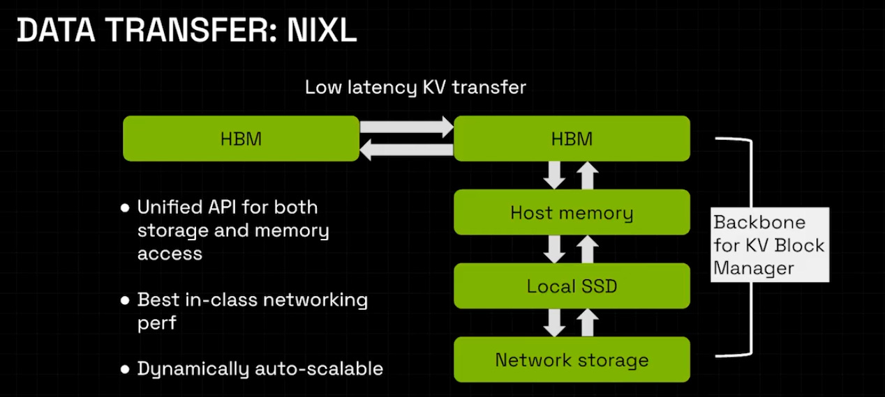
The NIXL library, which provides an asynchronous peer-to-peer transfer API for moving data, such as KV-cache, between prefill and decode machines and across memory hierarchies. The async behavior is important because it lets communication overlap with computation. This differs from NCCL, which is mainly designed for collective operations and is not asynchronous.
Source: NVIDIA An AI Configurator, which recommends the best deployment setup (cluster size, parallelism strategies, and so on) based on the model and latency requirements.


Rubin CPX
This finally brings us to Rubin CPX. In my article Three examples of how ASICs and FPGAs are used as accelerators, I describe a recurring pattern in engineering: whenever possible, software optimizations transition into specialized hardware. With NVIDIA Dynamo and inference engines like vLLM pushing the industry toward disaggregated inference, the logical next step is to formalize the architecture and build hardware tailored to the use-case rather than relying on general-purpose GPUs, and Rubin CPX is exactly that.
To appreciate the capabilities of this new processor, it helps to compare it with NVIDIA’s broader GPU lineup. A quick look at the spec sheet shows that Rubin CPX isn’t a watered-down B200 or Rubin GPU. It’s much closer to an enhanced version of the NVIDIA RTX 6000 PRO Blackwell workstation-class GPU.
This is evident from the inclusion of NVENC/NVDEC video engines (to accelerate video generation workloads). Primary connectivity is PCIe and there’s no NVLink. The memory is GDDR7 and not HBM. Let’s dig into these further.
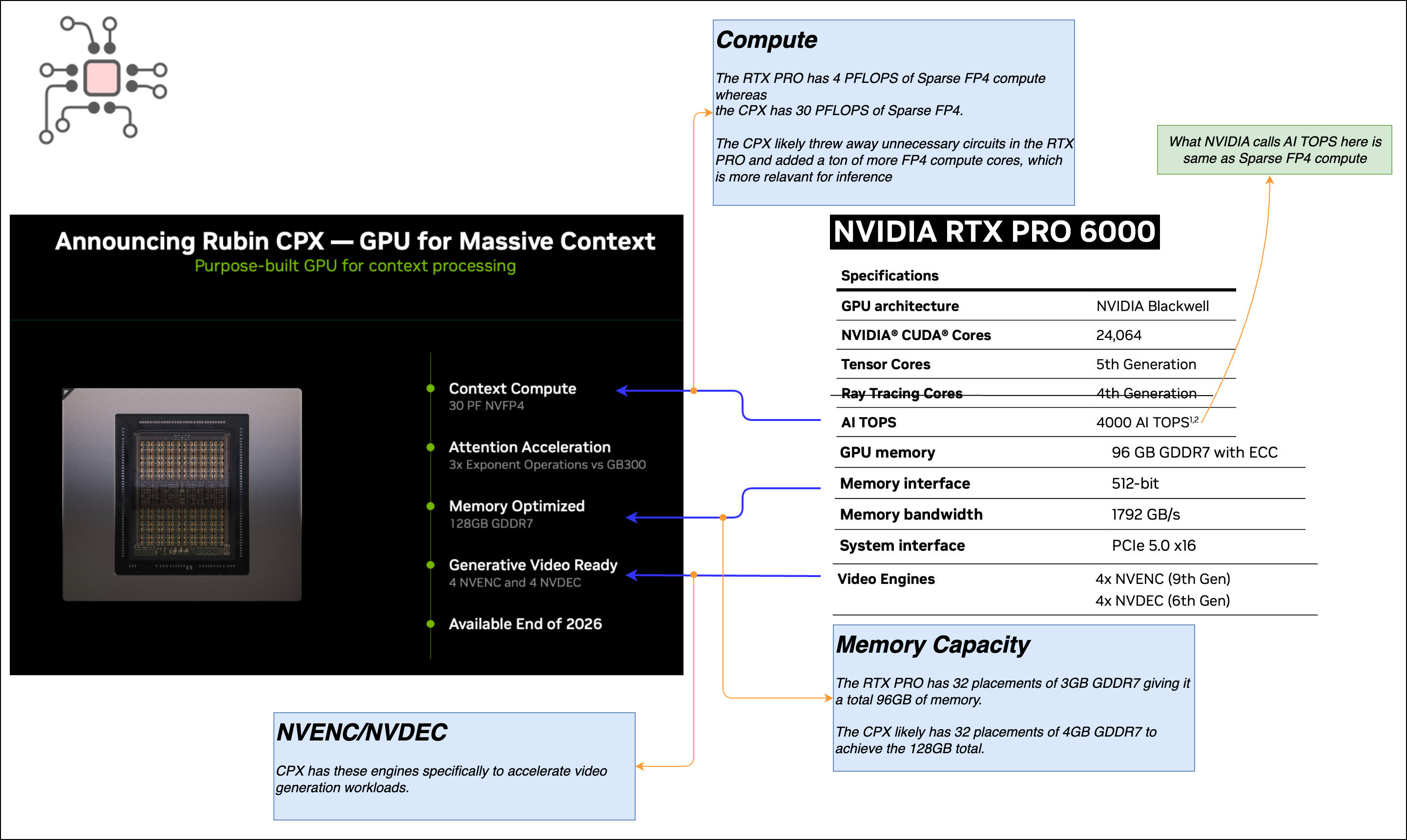
Compute

This CPX delivers 30 PFLOPS of sparse FP4 compute, which is substantial considering the dual-die Rubin GPU does 50 PFLOPS. So, on a per-die basis, the CPX provides more FP4 compute than a single Rubin GPU die.